Informatica Training & Tutorials

Informatica PowerCenter Workflows on Grid for Performance and Scalability

Informatica has developed a solution that leverages the power of grid computing for greater data integration scalability and performance. The grid option delivers the load balancing, dynamic partitioning, parallel processing and high availability to ensure optimal scalability, performance and reliability. In this article lets discuss how to setup Infrmatica Workflow to run on grid.

What is PowerCenter On Grid

When a PowerCenter domain contains multiple nodes, you can configure workflows and sessions to run on a grid. When you run a workflow on a grid, the Integration Service runs a service process on each available node of the grid to increase performance and scalability. When you run a session on a grid, the Integration Service distributes session threads to multiple DTM processes on nodes in the grid to increase performance and scalability.

Domain : A PowerCenter domain consists of one or more nodes in the grid environment. PowerCenter services run on the nodes. A domain is the foundation for PowerCenter service administration.

Node : A node is a logical representation of a physical machine that runs a PowerCenter service.

Admin Console with Grid Configuration

Below shown is an Informatica Admin Console, with two node Grid configuration. We can see two nodes Node_1, Node_2 and the Node_GRID grid created using two nodes. The integration service Int_service_GRID is running on the grid.

Setting up Workflow on Grid

When you setup a workflow to run grid, the Integration Service distributes workflows across the nodes in a grid. It also distributes the Session, Command, and predefined Event-Wait tasks within workflows across the nodes in a grid.

You can setup the workflow to run on grid as shown in below image.You can assign the integration service, which is configured on grid to run the workflow on grid.

Setting up Session on Grid

When you run a session on a grid, the Integration Service distributes session threads across nodes in a grid. The Load Balancer distributes session threads to DTM processes running on different nodes. You might want to configure a session to run on a grid when the workflow contains a session that takes a long time to run.

You can setup the session to run on grid as shown in below image.

Workflow Running on Grid

Below workflow monitor screen shots sows a workflow running on grid. You see two of the session in the workflow wf_Load_CUST_DIM run on Node_1 and other one on Node_1 from 'Task Progress Details' Window.

Key Features and Advantages of Grid

Load Balancing : While facing spikes in data processing, load balance guarantees smooth operations by switching the data processing between nodes on the grid. The node is chosen dynamically based on process size, CPU utilization, memory requirements etc...
High Availability : Grid complements the High Availability feature or PowerCenter by switching the master node in case of a node failure. This ensures the monitoring and the shorten time needed for recovery processes.
Dynamic Partitioning : Dynamic Partitioning helps making the best use of currently available nodes on the grid. By adapting to available resources, it also helps increasing the performance of the whole ETL process.

Hope you enjoyed this article, please leave us a comment or feedback if you have any, we are happy to hear from you.

Informatica PowerCenter Workflows runs on grid, distributes workflow tasks across nodes in the grid. It also distributes Session, Command, and predefined Event-Wait tasks within workflows across the nodes in a grid. PowerCenter uses load balancer to distribute workflows and session tasks to different nodes. This article describes, how to use load balancer to setup high workflow priorities and how to allocate resources.

What is Informatica Load Balancing

Informatica load Balancing is a mechanism which distributes the workloads across the nodes in the grid. When you run a workflow, the Load Balancer dispatches different tasks in the workflow such as Session, Command, and predefined Event-Wait tasks to different nodes running the Integration Service. Load Balancer matches task requirements with resource availability to identify the best node to run a task. It may dispatch tasks to a single node or across nodes on the grid.

Identifying the Nodes to Run a Task

Load Balancer matches the resources required by the task with the resources available on each node. It dispatches tasks in the order it receives them. You can adjust the workflow priorities and the assign resources needs for tasks, such that load balancer can distribute the tasks to the right nodes and right priority.

Assign service levels : You assign service levels to workflows. Service levels establish priority among workflow tasks that are waiting to be dispatched.

Assign resources : You assign resources to tasks. Session, Command, and predefined Event-Wait tasks require PowerCenter resources to succeed. If the Integration Service is configured to check resources, the Load Balancer dispatches these tasks to nodes where the resources are available.

Assigning Service Levels to Workflows

Service levels determine the order in which the Load Balancer dispatches tasks from the dispatch queue. When multiple tasks are waiting to be dispatched, the Load Balancer dispatches high priority tasks before low priority tasks. You create service levels and configure the dispatch priorities in the Administrator tool.

Integration service will be limited to run You give Higher Service Level for the workflows, which needs to be dispatched first, when multiple workflows are running in parallel. Service Levels are set up in the Admin console.

You assign service levels to workflows on the General tab of the workflow properties as shown below.

Informatica PowerCenter Load Balancing for Workload Distribution on Grid

Assigning Resources to Tasks

If the Integration Service runs on a grid and is configured to check for available resources, the Load Balancer uses resources to dispatch tasks. The Integration Service matches the resources required by tasks in a workflow with the resources available on each node in the grid to determine which nodes can run the tasks.

You can configure the resource requirements by the tasks as shown in below image.

Below configuration shows that, the source qualifier needs source file from File DirectoryNDMSource, which is accessible only from one node. Available resource on different nodes are configured from Admin console.

Hope you enjoyed this article and this will help you prioritize your workflows to to meet your data refresh time lines. Please leave us a comment or feedback if you have any, we are happy to hear from you.

Surrogate Key in Data Warehouse, What, When, Why and Why Not

Surrogate keys are widely used and accepted design standard in data warehouses. It is sequentially generated unique number attached with each and every record in a Dimension table in any Data Warehouse. It join between the fact and dimension tables and is necessary to handle changes in dimension table attributes.

What Is Surrogate Key

Surrogate Key (SK) is sequentially generated meaningless unique number attached with each and every record in a table in any Data Warehouse (DW).

It is UNIQUE since it is sequentially generated integer for each record being inserted in the table.
It is MEANINGLESS since it does not carry any business meaning regarding the record it is attached to in any table.
It is SEQUENTIAL since it is assigned in sequential order as and when new records are created in the table, starting with one and going up to the highest number that is needed.

Surrogate Key Pipeline and Fact Table

During the FACT table load, different dimensional attributes are looked up in the corresponding Dimensions and SKs are fetched from there. These SKs should be fetched from the most recent versions of the dimension records. Finally the FACT table in DW contains the factual data along with corresponding SKs from the Dimension tables.

The below diagram shows how the FACT table is loaded from the source. Surrogate Key in Data Warehouse, What, When, Why and Why Not

Why Should We Use Surrogate Key

Basically it’s an artificial key that is used as a substitute for a Natural Key (NK). We should have defined NK in our tables as per the business requirement and that might be able to uniquely identify any record. But, SK is just an Integer attached to a record for the purpose of joining different tables in a Star or Snowflake schema based DW. SK is much needed when we have very long NK or the datatype of the NK is not suitable for Indexing.

The below image shows a typical Star Schema, joining different Dimensions with the Fact using SKs.

Ralph Kimball emphasizes more on the abstraction of NK. As per him, Surrogate Keys should NOT be:

Smart, where you can tell something about the record just by looking at the key.
Composed of natural keys glued together.
Implemented as multiple parallel joins between the dimension table and the fact table; so-called double or triple barreled joins.

As per Thomas Kejser, a “good key” is a column that has the following properties:

It forced to be unique
It is small
It is an integer
Once assigned to a row, it never changes
Even if deleted, it will never be re-used to refer to a new row
It is a single column
It is stupid
It is not intended as being remembered by users

If the above mentioned features are taken into account, SK would be a great candidate for a Good Key in a DW.

Apart from these, few more reasons for choosing this SK approach are:

If we replace the NK with a single Integer, it should be able to save a substantial amount of storage space. The SKs of different Dimensions would be stored as Foreign Keys (FK) in the Fact tables to maintain Referential Integrity (RI), and here instead of storing of those big or huge NKs, storing of concise SKs would result in less amount of space needed. The UNIQUE indexes built on the SK will take less space than the UNIQUE index built on the NK which may be alphanumeric.
Replacing big, ugly NKs and composite keys with beautiful, tight integer SKs is bound to improve join performance, since joining two Integer columns works faster. So, it provides an extra edge in the ETL performance by fastening data retrieval and lookup.
Advantage of a four-byte integer key is that it can represent more than 2 billion different values, which would be enough for any dimension and SK would not run out of values, not even for the Big or Monster Dimension.
SK is usually independent of the data contained in the record, we cannot understand anything about the data in a record simply by seeing only the SK. Hence it provides Data Abstraction.

So, apart from the abstraction of critical business data involved in the NK, we have the advantage of storage space reduction as well to implement the SK in our DW. It has become a Standard Practice to associate an SK with a table in DW irrespective of being it a Dimension, Fact, Bridge or Aggregate table.

Why Shouldn’t We Use Surrogate Key

There are myriad number of disadvantages as well while working with SK. Let’s see them one by one:

The values of SKs have no relationship with the real world meaning of the data held in a row. Therefore over usage of SKs lead to the problem of disassociation.
The generation and attachment of SK creates unnecessary ETL burden. Sometimes it may be found that the actual piece of code is short and simple, but generating the SK and carrying it forward till the target adds extra overhead on the code.
During the Horizontal Data Integration (DI) where multiple source systems loads data into a single Dimension, we have to maintain a single SK Generating Area to enforce the Uniqueness of SK. This may come as an extra overhead on the ETL.
Even query optimization becomes difficult since SK takes the place of PK, unique index is applied on that column. And any query based on NK leads to Full Table Scan (FTS) as that query cannot take the advantage of unique index on the SK.
Replication of data from one environment to another, i.e. Data Migration, becomes difficult since SKs from different Dimension tables are used as the FKs in the Fact table and SKs are DW specific, any mismatch in the SK for a particular Dimension would result in no data or erroneous data when we join them in a Star Schema.
If duplicate records come from the source, there is a potential risk of duplicates being loaded into the target, since Unique Constraint is defined on the SK and not on the NK.

About the Author

Crux of the matter is that SK should not be implemented just in the name of standardizing your code. SK is required when we cannot use an NK to uniquely identify a record or when using an SK seems more suitable as the NK is not a good fit for PK.

Different Approaches to Generate Surrogate Key in Informatica PowerCenter

Surrogate Key is sequentially generated unique number attached with each and every record in a Dimension table in any Data Warehouse. We discussed about Surrogate Key in in detail in our previous article. Here in this article we will concentrate on different approaches to generate Surrogate Key for different type ETL process.

Surrogate Key for Dimensions Loading in Parallel

When you have a single dimension table loading in parallel from different application data sources, special care should be given to make sure that no keys are duplicated. Lets see different design options here.

1. Using Sequence Generator Transformation

This is the simplest and most preferred way to generate Surrogate Key(SK). We create a reusable Sequence Generator transformation in the mapping and map the NEXTVAL port to the SK field in the target table in the INSERT flow of the mapping. The start value is usually kept 1 and incremented by 1.

Below shown is a reusable Sequence Generator transformation.

NEXTVAL port from the Sequence Generator can be mapped to the surrogate key in the target table. Below shown is the sequence generator transformation.

Note : Make sure to create a reusable transformation, so that the same transformation can be reused in multiple mappings, which loads the same dimension table.

2. Using Database Sequence

We can create a SEQUENCE in the database and use the same to generate the SKs for any table. This can be invoked by a SQL Transformation or a using a Stored Procedure Transformation.

First we create a SEQUENCE using the following command.

CREATE SEQUENCE DW.Customer_SK
MINVALUE 1
MAXVALUE 99999999
START WITH 1
INCREMENT BY 1;

Using SQL Transformation

You can create a create reusable reusable SQL Transformation as shown below. It takes the name of the database sequence and the schema name as input and returns SK numbers.

Schema name (DW) and sequence name (Customer_SK) can be passed in as input value for the transformation and the output can be mapped to the target SK column. Below shown is the SQL transformation image.

Using Stored Procedure Transformation

We use the SEQUENCE DW.Customer_SK to generate the SKs in an Oracle function, which in turn called via a stored procedure transformation.

Create a database function as below. Here we are creating an Oracle function.

CREATE OR REPLACE FUNCTION DW.Customer_SK_Func
RETURN NUMBER
IS
Out_SK NUMBER;
BEGIN
SELECT DW.Customer_SK.NEXTVAL INTO Out_SK FROM DUAL;
RETURN Out_SK;
EXCEPTION
WHEN OTHERS THEN
raise_application_error(-20001,'An error was encountered - '||SQLCODE||' -ERROR- '||SQLERRM);
END;

You can import the database function as a stored procedure transformation as shown in below image.

Now, just before the target instance for Insert flow, we add an Expression transformation. We add an output port there with the following formula. This output port GET_SK can be connected to the target surrogate key column.

GET_SK =:SP. CUSTOMER_SK_FUNC()

Note : Database function can be parametrized and the stored procedure can also be made reusable to make this approach more effective

Surrogate Key for Non Parallel Loading Dimensions

If the dimension table is not loading in parallel from different application data sources, we have couple of more options to generate SKs. Lets see different design options here.

Using Dynamic LookUP

When we implement Dynamic LookUP in any mapping, we may not even need to use the Sequence Generator for generating the SK values.

For a Dynamic LookUP on Target, we have the option of associating any LookUP port with an input port, output port, or Sequence-ID. When we associate a Sequence-ID, the Integration Service generates a unique Integer value for each inserted rows in the lookup cache., but this is applicable for the ports with Bigint, Integer or Small Integer data type. Since SK is usually of Integer type, we can exploit this advantage.

The Integration Service uses the following process to generate Sequence IDs.

When the Integration Service creates the dynamic lookup cache, it tracks the range of values for each port that has a sequence ID in the dynamic lookup cache.
When the Integration Service inserts a row of data into the cache, it generates a key for a port by incrementing the greatest sequence ID value by one.
When the Integration Service reaches the maximum number for a generated sequence ID, it starts over at one. The Integration Service increments each sequence ID by one until it reaches the smallest existing value minus one. If the Integration Service runs out of unique sequence ID numbers, the session fails.

Above shown is a dynamic lookup configuration to generate SK for CUST_SK.

The Integration Service generates a Sequence-ID for each row it inserts into the cache. For any records which is already present in the Target, it gets the SK value from the Target Dynamic LookUP cache, based on the Associated Ports matching. So, if we take this port and connect to the target SK field, there will not be any need to generate SK values separately, since the new SK value(for records to be Inserted) or the existing SK value(for records to be Updated) is supplied from the Dynamic LookUP.

The disadvantage of this technique lies in the fact that we don’t have any separate SK Generating Area and the source of SK is totally embedded into the code.

Using Expression Transformation

Suppose we are populating a CUSTOMER_DIM. So in the Mapping, first create a Unconnected Lookup for the dimension table, say LKP_CUSTOMER_DIM. The purpose is to get the maximum SK value in the dimension table. Say the SK column is CUSTOMER_KEY and the NK column is CUSTOMER_ID.

Select CUSTOMER_KEY as Return Port and Lookup Condition as

CUSTOMER_ID = IN_CUSTOMER_ID

Use the SQL Override as below:

SELECT MAX (CUSTOMER_KEY) AS CUSTOMER_KEY, '1' AS CUSTOMER_ID FROM CUSTOMER_DIM

Next in the mapping after the SQ use an Expression transformation. Here actually we will be generating the SKs for the Dimension based on the previous value generated. We will create the following ports in the EXP to compute the SK value.

VAR_COUNTER = IIF(ISNULL( VAR_INC ), NVL(:LKP.LKP_CUSTOMER_DIM('1'), 0) + 1, VAR_INC + 1 )

VAR_INC = VAR_COUNTER

OUT_COUNTER = VAR_COUNTER

When the mapping starts, for the first row we will look up the Dimension table to fetch the maximum available SK in the table. Next we will keep on incrementing the SK value stored in the variable port by 1 for each incoming row. Here the O_COUNTER will give the SKs to be populated in CUSTOMER_KEY.

Using Mapping & Workflow Variable

Here again we will use the Expression transformation to compute the next SK, but will get the MAX available SK in a different way.

Suppose, we have a session s_New_Customer, which loads the Customer Dimension table. Before that session in the Workflow, we add a dummy session as s_Dummy.

In s_Dummy, we will have a mapping variable, e.g. $$MAX_CUST_SK which will be set with the value of MAX (SK) in Customer Dimension table.

SELECT MAX (CUSTOMER_KEY) AS CUSTOMER_KEY FROM CUSTOMER_DIM

We will have the CUSTOMER_DIM as our source table and target can be a simple flat file, which will not be used anywhere. We pull this MAX (SK) from the SQ and then in an EXP we assign this value to the mapping variable using the SETVARIABLE function. So, we will have the following ports in the EXP:

INP_CUSTOMER_KEY = INP_CUSTOMER_KEY -– The MAX of SK coming from Customer Dimension table.
OUT_MAX_SK = SETVARIABLE ($$MAX_CUST_SK, INP_CUSTOMER_KEY) –- Output Port

This output port will be connected to the flat file port, but the value we assigned to the variable will persist in the repository.

In our second mapping we start generating the SK from the value $$MAX_CUST_SK + 1. But how can we pass the parameter value from one session into the other one?

Here the use of Workflow Variable comes into picture. We define a WF variable as $$MAX_SK and in the Post-session on success variable assignment section of s_Dummy, we assign the value of $$MAX_CUST_SK to $$START_SK. Now the variable $$MAX_SK contains the maximum available SK value from CUSTOMER_DIM table. Next we define another mapping variable in the session s_New_Customer as $$START_VALUE and this is assigned the value of $$MAX_SK in the Pre-session variable assignment section of s_New_Customer.

So, the sequence is:

Post-session on success variable assignment of First Session:

$$MAX_SK = $$MAX_CUST_SK

Pre-session variable assignment of Second Session:

$$START_VALUE = $$MAX_SK

Now in the actual mapping, we add an EXP and the following ports into that to compute the SKs one by one for each records being loaded in the target.

VAR_COUNTER = IIF (ISNULL (VAR_INC), $$START_VALUE + 1, VAR_INC + 1)
VAR_INC = VAR_COUNTER
OUT_COUNTER = VAR_COUNTER

About the Author

OUT_COUNTER will be connected to the SK port of the target.

Hope you enjoyed this article and earned some new ways to generate surrogate keys for your dimension tables. Please leave us a comment or feedback if you have any, we are happy to hear from you.

Informatica Performance Tuning Guide, Performance Enhancements - Part 4

In our performance turning article series, so far we covered about the performance turning basics, identification of bottlenecks and resolving different bottlenecks. In this article we will cover different performance enhancement features available in Informatica PowerCener. In addition to the features provided by PowerCenter, we will go over the designs tips and tricks for ETL load performance improvement.

Performance Enhancements Features

The main PowerCenter features for Performance Enhancements are.

Performance Tuning Tutorial Series
Part I : Performance Tuning Introduction.
Part II : Identify Performance Bottlenecks.
Part III : Remove Performance Bottlenecks.
Part IV : Performance Enhancements.

Pushdown Optimization.
Pipeline Partitions.
Dynamic Partitions.
Concurrent Workflows.
Grid Deployments.
Workflow Load Balancing.
Other Performance Tips and Tricks.

1. Pushdown Optimization

Pushdown Optimization Option enables data transformation processing, to be pushed down into any relational database to make the best use of database processing power. It converts the transformation logic into SQL statements, which can directly execute on database. This minimizes the need of moving data between servers and utilizes the power of database engine.

Read More about Pushdown Optimization.

2. Session Partitioning

The Informatica PowerCenter Partitioning Option increases the performance of PowerCenter through parallel data processing. Partitioning option will let you split the large data set into smaller subsets which can be processed in parallel to get a better session performance.

Read More about Session Partitioning.

3. Dynamic Session Partitioning

Informatica PowerCenter session partition can be used to process data in parallel and achieve faster data delivery. Using Dynamic Session Partitioning capability, PowerCenter can dynamically decide the degree of parallelism. The Integration Service scales the number of session partitions at run time based on factors such as source database partitions or the number of CPUs on the node resulting significant performance improvement.

Read More about Dynamic Session Partition.

4. Concurrent Workflows

A concurrent workflow is a workflow that can run as multiple instances concurrently. A workflow instance is a representation of a workflow. We can configure two types of concurrent workflows. It can be concurrent workflows with the same instance name or unique workflow instances to run concurrently.

Read More about Concurrent Workflows.

5. Grid Deployments

Read More about Grid Deployments.

6. Workflow Load Balancing

Informatica Load Balancing is a mechanism which distributes the workloads across the nodes in the grid. When you run a workflow, the Load Balancer dispatches different tasks in the workflow such as Session, Command, and predefined Event-Wait tasks to different nodes running the Integration Service. Load Balancer matches task requirements with resource availability to identify the best node to run a task. It may dispatch tasks to a single node or across nodes on the grid.

Read More about Workflow Load Balancing.

7. Other Performance Tips and Tricks

Through out this blog we have been discussing different tips and tricks to improve your ETL load performance. We would like to reference those tips and tricks in this article for your reference.

Read More about Other Performance Tips and Tricks.

Hope you guys enjoyed these tips and tricks and it is helpful for your project needs. Leave us your questions and commends. We would like to hear any other performance tips you might have used in your projects.

In our couple of prior articles we spoke about change data capture, different techniques to capture change data and a change data capture frame work as well. In this article we will deep dive into different aspects for change data in Data Warehouse including soft and hard deletions in source systems.

Revisiting Change Data Capture (CDC)

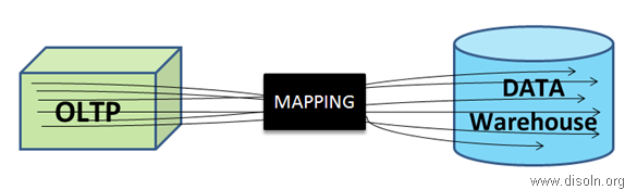
When we talk about Change Data Capture (CDC) in DW, we mean to capture those changes that have happened at the source side so far after we have run our job last time. In Informatica we call our ETL code as ‘Mapping’, because we MAP the source data (OLTP) into the target data (DW) and the purpose of running the ETL codes is to keep the source and target data in sync, along with some transformations in between, as per the business rules.

SOFT and HARD Deleted Records and Change Data Capture in Data Warehouse

Now, data may get changed at source in three different ways.

NEW transactions happened at source.
CORRECTIONS happened on old transactional values or measured values.
INVALID transactions removed from source.

Usually in our ETL we take care of the 1st and 2nd case(Insert/Update Logic); the 3rd change is not captured in DW unless it is specifically instructed in the requirement specification. But when it’s especially amended, we need to devise convenient ways to track the transactions that were removed i.e., to track the deleted records at source and accordingly DELETE those records in DW.

One thing to make clear is that Purging might be enabled at your OLTP, i.e OLTP keeping data for a fixed historical period of time, but that is a different scenario. Here we are more interested about what was DELETED at Source because the transactions was NOT valid.

Effects in DW for Source Data Deletion

DW tables can be divided into three categories as related to the deleted source data.

When the DW table load nature is 'Truncate & Load' or 'Delete & Reload', we don't have any impact, since the requirement is to keep the exact snapshot of the source table at any point of time.
When the DW table does not track history on data changes and deletes are allowed against the source table. If a record is deleted in the source table, it is also deleted in the DW.
When the DW table tracks history on data changes and deletes are allowed against the source table. The DW table will retain the record that has been deleted in the source system, but this record will be either expired in DW based on the change captured date or 'Soft Delete' will be applied against it.

Types of Data Deletion

Academically, deleting records from DW table is forbidden, however, it’s a common practice in most DWs when we face this kind of situations. Again, if we are deleting records from DW, it has to be done after proper discussions with Business. If your Business requires DELETION, then there are two ways.

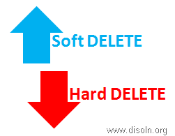
Logical Delete :- In this case, we have a specific flag in the source table as STATUS which would be having the values as ‘ACTIVE’ or ‘INACTIVE’. Some OLTPs keep the field name as ACTIVE with the values as ‘I’, ‘U’ or ‘D’, where ‘D’ means that the record is deleted or the record is INACTIVE. This approach is quite safe and also known as Soft DELETE.

Physical Delete :- In this case the record related to invalid transactions are fully deleted from the source table by issuing DML statement. This is usually done after thorough discussing with Business Users and related business rules are strictly followed. This is also known as Hard DELETE.

ETL Perspective on Deletion

When we have ‘Soft DELETE’ implemented at the source side, it becomes very easy to track the invalid transactions and we can tag those transactions in DW accordingly. We just need to filter the records from source using that STATUS field and issue an UPDATE in DW for the corresponding records. Few things to be kept in mind in this case.

If only ACTIVE records are supposed to be used in ETL processing, we need to add specific filters while fetching source data.

Sometimes INACTIVE records are pulled into the DW and moved till the ETL Data Warehouse level. While pushing the data into Exploration Data Warehouse, only the ACTIVE records are sent for reporting purpose.

For ‘Hard DELETE’, if Audit Table is maintained at source systems for what are transactions were deleted, we can source the same, i.e. join the Audit table and the Source table based on NK and logically delete them in DW too. But it becomes quite cumbersome and costly when no account is kept of what was deleted at all. In these cases, we need to use different ways to track them and update the corresponding records in DW.

Deletion in Data Warehouse : Dimension Vs Fact

In most of the cases, we see only the transactional records to be deleted from source systems. DELETION of Data Warehouse records are a rare scenario.

Deletion in Dimension Tables

If we have DELETION enabled for Dimensions in DW, it's always safe to keep a copy of the OLD record in some AUDIT table, as it helps to track any defects in future. A simple DELETE trigger should work fine; since DELETION hardly happens, this trigger would not degrade the performance much.

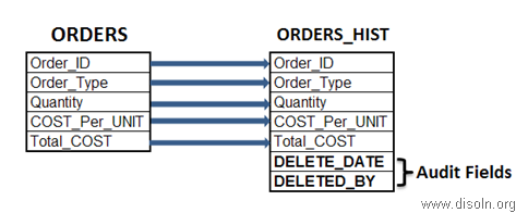
Let's take this ORDERS table into consideration. Along with this, we can have a History table for ORDERS, e.g. ORDERS_Hist, which would store the DELETED records from ORDERS.

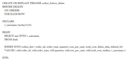
The below Trigger will work fine to achieve this.

The AUDIT Fields will convey when this particular record was deleted and by which user. But this table needs to be created for each and every DW table where we want to keep the audit of what was DELETED. If the entire record is not need and only fields involved in Natural Key(NK) may work, we can have a consolidated table for all the Dimensions.

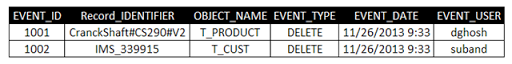
Here the Record_IDENTIFIER field contains the values of all the columns involved in the Natural Key(NK) separated by '#' of the table mentioned in the OBJECT_NAME field.

Sometimes, we face a situation in DW where a FACT table record contains a Surrogate Key(SK) from a Dimension but the Dimension table doesn't own it anymore. In those cases, the FACT table record becomes orphan and it will hardly be able to appear in any report since we always use the INNER JOIN between Dimensions and Fact while retrieving data in the reporting layer, and there it misses the Referential Integrity(RI).

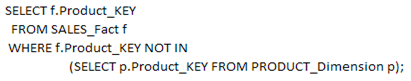
Suppose, we want to track the orphan records from the SALES Fact table in respect of Product Dimension. We can use the query as below.

So, the above query will provide only the Orphan records, BUT certainly it cannot provide you the records DELETED from the PRODUCT_Dimension. So, one feasible solution could be while populating the EVENT table with the SKs from PRODUCT_Dimension that are being DELETED, provided we don't reuse our Surrogate Keys. So, when we have both the SKs and the NKs from the PRODUCT_Dimension in the EVENT table for DELETED entries, we can achieve a better compliance over the Data Warehouse data.

Another useful but least used approach is enabling the audit for any table for DELETE in an Oracle DB using queries like the following.

Audit DELETE on SCHEMA.TABLE;

The table DBA_AUDIT_STATEMENT will contain all the related details related to this deletion, example the user who issued the, exact DML statement and so on, but this cannot provide you with the record that was deleted. Since this approach cannot directly provide you information on which record was deleted, it’s not so useful in our current discussion, so I would like to keep aloof from the topic here.

Deletion in Fact Tables

Now, this was all about DELETION in DW Dimension tables. Regarding FACT data DELETION, I would like to cite an extract of what Ralph Kimball has to say on Physical Deletion of Facts from DW.

Change Data Capture & Apply for 'Hard DELETE' in Source

Again, whether we should track the DELETED records from source or not depends on the type of table and its Load Nature. I will share few genuine scenarios that are usually faced in any DW and discuss about the solutions accordingly.

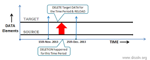
1. Records are DELETED from SOURCE for a known Time Period, no Audit Trail was kept.

In this case, the ideal solution is to DELETE the entire records’ set in DW for the Target table and pull the source records once again for the time period. This will bring the DW in sync with Source and DELETED records also will not be available in DW.

Usually time period is mentioned in terms of Ship_DATE or Invoice_DATE or Event_DATE, i.e. a DATE type field from the actual dataset of the source table is used, and hence the way we can filter the records for Extraction from source table using WHERE clause, we can do the same in DW table as well.

Obviously, in this case we are NOT able to capture the 'Hard DELETE' from the Source i.e., we cannot track the History of DATA, but we would be able to bring the Source and DW in sync at the least. Again, this approach is recommended only when the situation occurs once in a while and not on regular basis.

2. Records are DELETED from SOURCE on regular basis with NO Timeframe, no Audit Trail was kept.

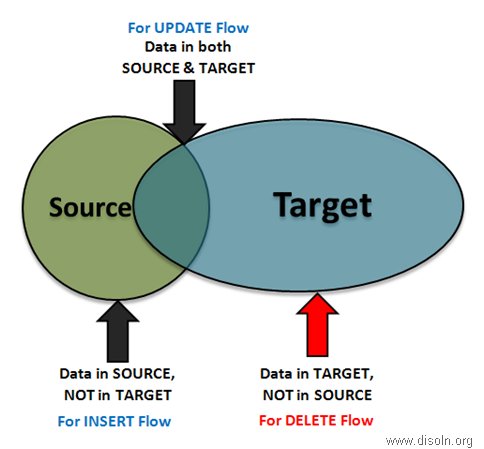
The possible solution in this case would be to implement FULL Outer JOIN between the Source and the Target table. The tables should be joined on the fields involved in the Natural Key(NK). This approach will help us to track all three kinds of changes to source data in one shot.

The logic can be better explained with the help of a Venn diagram.

Out of the Joiner (kept in FULL Outer Join mode),

Records that have values for the NK fields only from the Source and not from the Target, they should go for the INSERT flow. These are all new records coming from source.
Records that have values for the NK fields from both the Source and the Target, they should go for the UPDATE flow. These are already existing records of Source.
Records that have values for the NK fields only from Target, will go for the DELETE flow. These are the records that were somehow DELETED from Source table.

Now, what we do with those DELETED records from Source, i.e. apply 'Soft DELETE' or 'Hard DELETE' in DW, depends on our requirement specification and business scenarios.

But this approach is having severe disadvantage in terms of ETL Performance. Whenever we go for a FULL Outer JOIN between Source and Target, we are using the entire data set from both the ends and this will obviously obstruct the smooth processing of ETL when data volume increases.

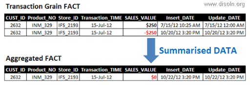
3. Records are DELETED from SOURCE, Audit Trail was kept.

Even though I'm mentioning it a DELETION, it's NOT the kind of Physical DELETION that we discussed previously. This is mainly related to incorrect transactions in Legacy Systems, e.g. Mainframes, which usually send data in flat files.

When some old transactions become invalidated, source team sends those transactions related records again to DW but with inverted measures, i.e. the sales figure are same as the old ones but they are negative. So, DW contains both the old set of records and the newly arrived records, but the aggregated measures become NULL in the aggregated FACT table, thus diminishing the impact of those invalid transactions in DW to NULL.

Only disadvantage of this approach is, Aggregated FACT contains the correct data at the summarized level, but the transactional FACT dual set of records, which together

About the Author

represent the real scenario, i.e. at first the transaction happened(with the older record) and then it became invalid(with the newer record).

Hope you guys enjoyed this article and gave you some new insights into change data capture in Data Warehouse. Leave us your questions and commends. We would like to hear how you have handled change data capture in your data warehouse.

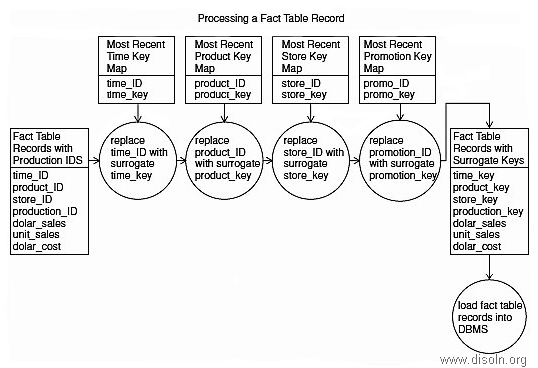
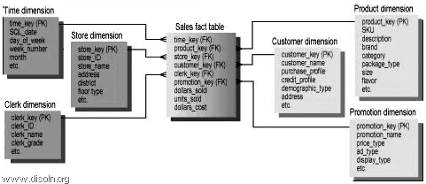
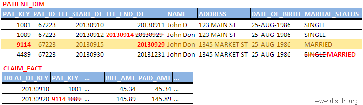
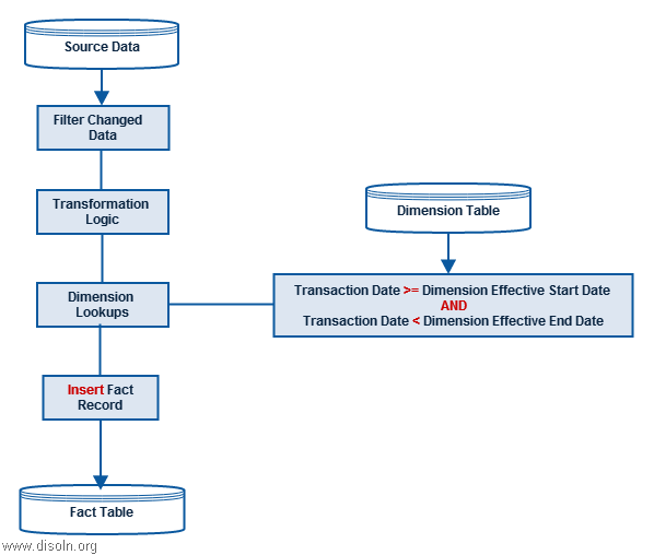
Design Approach to Handle Late Arriving Dimensions and Late Arriving Facts

In the typical case for a data warehouse, dimensions are processed first and the facts are loaded later, with the assumption that all required dimension data is already in place. This may not be true in all cases because of nature of your business process or the source application behavior. Fact data also, can be sent from the source application to the warehouse way later than the actual fact data is created. In this article lets discusses several options for handling late arriving dimension and Facts.

What is Late Arriving Dimension

Late arriving dimensions or sometimes called early-arriving facts occur when you have dimension data arriving in the data warehouse later than the fact data that references that dimension record.

For example, an employee availing medical insurance through his employer is eligible for insurance coverage from the first day of employment. But the employer may not provide the medical insurance information to the insurance provider for several weeks. If the employee undergo any medical treatment during this time, his medical claim records will come as fact records with out having the corresponding patient dimension details.

Design Approaches

Depending on the business scenario and the type of dimension in use, we can take different design approaches.

Hold the Fact record until Dimension record is available.
'Unknown' or default Dimension record.
Inferring the Dimension record.
Late Arriving Dimension and SCD Type 2 changes.

1. Hold the Fact record until Dimension record is available

One approach is to place the fact row in a suspense table. The fact row will be held in the suspense table until the associated dimension record has been processed. This solution is relatively easy to implement, but the primary drawback is that the fact row isn’t available for reporting until the associated dimension record has been handled.

This approach is more suitable when your data warehouse is refreshed as a scheduled batch process and a delay in loading fact records until the dimension records are available is acceptable for the business.

2. 'Unknown' or default Dimension record

Another approach is to simply assign the “Unknown” dimension member to the fact record. On the positive side, this approach does allow the fact record to be recorded during the ETL process. But it won’t be associated with the correct dimension value.

The "Unknown" fact records can also be kept into a suspense table. Eventually, when the Dimension data is processed, the suspense data can be reprocessed and associate with a real, valid Dimension record.

3. Inferring the Dimension record

Another method is to insert a new Dimension record with a new surrogate key and use the same surrogate key to load the incoming fact record. This only works if you have enough details about the dimension in the fact record to construct the natural key. Without this, you would never be able to go back and update this dimension row with complete attributes.

In the insurance claim example explained in the beginning; it is almost certain that the "patient id" will be part of the claim fact, which is the natural key of the patient dimension. So we can create a new placeholder dimension record for the patient with a new surrogate key and the natural key "patient id".

Note : When you get all other attributes for the patient dimension record in a later point, you will have to do a SCD Type 1 update for the first time and SCD Type 2 going forward.

4. Late Arriving Dimension and SCD Type 2 changes

Late arriving dimension with SCD Type 2 changes gets more complex to handle.

4.1. Late Arriving Dimension with multiple historical changes

As described above, we can handle late arriving dimension by keeping an "Unknown" dimension record or an "Inferred" dimension record, which acts an a placeholder.

Even before we get the full dimension record details from the source system, there may be multiple SCD Type 2 changes to the placeholder dimension record. This leads to the creation of new dimension record with new surrogate key and modify any subsequent fact records surrogate key to point the new surrogate key.

Lets see the scenario in detail with the help medical insurance claim example.

The patient with ID 67223 have made two insurance claims. One on 9/10 and other on 9/20. As there is no patient dimension information is available for patient id 67223 yet, an 'Inferred' dimension record is created for the patient with surrogate key 1001.

Below shown is the state of the dimension and the fact table at this point.

Later, by the time dimension information is made available, there has already been SCD Type 2 changes for the patient id 67223. There has been changes for the patient id 67223 on 9/10 and again on 9/12. Below shown is the current state of the dimension and fact records. The fact record created on 9/20 is still referring to surrogate key 1001, which is not the correct representation.

This means the claim record created on 9/20 need to be reassigned to the correct surrogate key, which is active for the same time period. Below shown is the correct state of the dimension and fact records.

4.2. Late Arriving Dimension with retro effective changes

You can get Dimension records from source system with retro effective dates. For example you might update your marital status in your HR system way later than your marriage date. This update come to data warehouse with retro effective date.

This leads to a new dimension record with a new surrogate key and changes in effective dates for the affected dimension. You will have to scan forward in the dimension to see if there is any subsequent type 2 rows for this dimension. This further leads in modify any subsequent fact records surrogate key to point the new surrogate key.

Lets again use the medical insurance claim example for our explanation.

Below shown state of the Patient Dimension and the Claim Fact table at this point, which is perfectly good.

Now we have got a Patient Dimension data from the source system say on 10/1, which is in effective from 9/15 as shown below.

This new Dimension data which comes with a retro effective date makes all dimension records out of sync in terms of the effective start and end date. In addition to that, the fact records are referring to incorrect dimension records.

So in addition to inserting a new dimension record with a new surrogate key, we will have to adjust the effective dates of the prior period dimension record and propagate the dimension column value changes to the remaining records. The fact table also need to be updated to reassign the correct surrogate key.

Below shown red is the corrections required to take care of the retro effective dimension records.

What is Late Arriving Facts

Late arriving fact scenario occurs when the transaction or fact data comes to data warehouse way later than the actual transaction occurred in the source application. If the late arriving fact need to be associated with an SCD Type 2 dimension, the situation become messy. This is because we have to search back in history within the dimensions to decide how to assign the right dimension keys that were in effect when the activity occurred in the past.

Design Approaches

Unlike late arriving dimensions, late arriving fact records can be handles relatively easily. When loading the fact record, the associated dimension table history has to be searched to find out the appropriate surrogate key which is effective at the time of the transaction occurrences. Below data flow describes the late arriving fact design approach.

Hope you guys enjoyed this article and gave you some new insights into late arriving dimension and fact scenarios in Data Warehouse. Leave us your questions and commends. We would also like to hear how you have handled late arriving dimension and fact in your data warehouse.

A high-level systematic ETL design will help to build efficient and flexible ETL processes. So special care should be given in the design phase of your project. In following we will be covering the key points one should keep in mind while designing an ETL process. The following recommendations can be integrated into your ETL design and development processes to simplify the effort and improve the overall quality of the finished product.

Consistency
Modularity
Reusability
Scalability
Simplicity

1. Consistency

To ensure consistency and facilitate easy maintenance post production it is important to define and agree on development standards before development work has begun.

The standards will define the ground rules for the development team. Standards can range in items from naming conventions to documentation standards to error handling standards. Development work should adhere to these standards throughout the life cycle and new team members will be able to reference these standards to understand the requirements placed upon the design and build activities

Applying consistent standards such as naming conventions, design patterns, error handling, change data capture reduces long term complications and makes maintenance easy.

2. Modularity

A modular design is important for an efficient ETL design. Divide different components of your ETL process such as incremental data pull logic, error handling, change data capture, operational meta data logging into different modules. This makes the ETL processes efficient, scalable, and maintainable.

3. Reusability

Reusability is a great feature in Informatica PowerCenter which can be used by developers. Its general purpose is to reduce unnecessary coding which ultimately reduces development time and increases supportability. In addition to that, it also help to react quickly to potential changes required for a program.

A great focus should be given during the design phase on reuse to make quick and universal modifications. Informatica PowerCenter has provided a variety of methods to achieve reusability such as Mapplets, Worklets, Reusable Transformations, Reusable functions, Parameters, Shared Folders.

4. Scalability

Keep volumes in mind in order to create efficient ETL process. Estimating the data volume requirements of a data integration project is a critical. Based on the volume estimates special consideration need to be given for caching different transformations, running complex queries, applying different performance turning techniques, such as push down optimization, Session Partitioning, Dynamic Session Partition, Concurrent Workflows, Grid Deployments, Workflow Load Balancing and Other available Performance Tips.

5. Simplicity

It is recommended to create multiple simple ETL Process, Informatica Mappings and Informatica Workflows instead of few complex ones. Use Staging Area and try to keep the processing logic as clear and simple as possible. Such design makes develop, debug, maintain easy compared to complex ETL logic.

Transaction Control Transformation to Control Commit and Rollback Transactions

In a typical Informatica PowerCenter workflow data is committed to the target table after a predefined number of rows are processed into target, which is specified in the session properties. But there are scenarios in which you need more control on the commits and rollbacks. In this article, lets see how we can achieve this using Transaction Control Transformation.

What is Transaction Control Transformation

A transaction is the set of rows bound by commit or roll back rows. The Transaction Control Transformation lets you control the commit and rollback transactions based on an expression or logic defined in the mapping. For example, you might want to define transactions based on a group of rows ordered on a common key, such as employee ID or order entry date.

When you run the session, the Integration Service evaluates the expression defined in the transformation for each row that enters the transformation. When it evaluates a commit row, it commits all rows in the transaction to the target. When the Integration Service evaluates a roll back row, it rolls back all rows in the transaction from the target.

Configuring Transaction Control Transformation

Transaction Control Transformation can be created and used as any other active transformations. All the required properties to configure this transformation can be provided in the Properties tab as shown in below image.

You can enter the transaction control expression in the Transaction Control Condition field. The transaction control expression uses the IIF function to test each row against the condition. The Integration Service evaluates the condition on a row-by-row basis. The return value determines whether the Integration Service commits, rolls back, or makes no transaction changes to the row.

You can use the following built-in variables in the Expression Editor when you create a transaction control expression.

TC_CONTINUE_TRANSACTION. The Integration Service does not perform any transaction change for this row. This is the default value of the expression.
TC_COMMIT_BEFORE. The Integration Service commits the transaction, begins a new transaction. The current row is in the new transaction.
TC_COMMIT_AFTER. The Integration Service writes the current row to the target, commits the transaction, and begins a new transaction. The current row is in the committed transaction.
TC_ROLLBACK_BEFORE. The Integration Service rolls back the current transaction, begins a new transaction. The current row is in the new transaction.
TC_ROLLBACK_AFTER. The Integration Service writes the current row to the target, rolls back the transaction, and begins a new transaction. The current row is in the rolled back transaction.

Transaction Control Transformation Use Case

Lets consider an ETL Job loading data into an OLTP application. The application data is being accessed by the system real time. This means the data loaded into the target table should confirm the consistency and integrity.

To be more specific about the use case, Sales order data loaded into the OLTP Application target table need to be committed after all the order items in a sales order is loaded into the target table.

Solution : Here lets create a Transaction Control Transformation, which is connected in the mapping pipeline after all the ETL logic is complete. The logic to define the commit points can be provided in the Transaction Control Transformation.

Step 1 :- Once the required transformation logic is build in the mapping, you create create a sorter transformation to group all the order items with in a sales order together based on ORDER_ID as shown in below.

Transaction Control Transformation to Control Commit and Rollback in Your ETL

Step 2 :- Create an expression transformation and add new ports with below expression. This step will let you identify, when all records in an order is complete processing.

V_NEXT_ORDER_FLAG (Variable) :- IIF(ORDER_ID = V_PRIOR_ORDER_ID, 'N', 'Y')
V_PRIOR_ORDER (Variable) :- ORDER_ID
NEXT_ORDER_FLAG (Output) :- V_NEXT_ORDER_FLAG

Hint :- This variable port technique can be used to preserve the value from a prior record.

Step 3 :- Now you can create the Transaction Control Transformation like any other active transformation and connect to the upstream transformation as shown below. Provide the expression to define the commit logic, below given is the expression per our use case.

IIF(NEXT_ORDER_FLAG = 'N',TC_CONTINUE_TRANSACTION,TC_COMMIT_BEFORE)

Step 4 :- Now you connect all the ports from Transaction Control transformation to the target definition.

Note :- While configuring the session, be sure to set the "Commit Type" Property as "User Defined"

Hope this tutorial was useful for your project. Please leave you questions and commends, We will be more than happy to help you.

You might have come across scenario where in you do not have enough good data in your Development and QA regions for your testing purpose; and you are not allowed to copy over data from production environment due to the data security reasons. Now using Informatica PowerCenter data masking transformation you can overcome such scenarios. In this article, lets see the usage of masking transformation.

What is Data Masking Transformation

Using Data Masking transformation, you change sensitive production data to realistic test data for non-production environments. The Data Masking transformation modifies source data based on masking rules that you configure for each column.

You can apply the following types of masking with the Data Masking transformation.

Key masking :- Produces deterministic results for the same source data,.
Random masking :- Produces random, non-repeatable results for the same source data.
Expression masking :- Applies an expression to a port to change the data or create data.
Substitution :- Replaces a column of data with similar but unrelated data from a dictionary.
Special mask formats :- Applies special mask formats to change SSN, credit card number, phone number, URL, email address, or IP addresses.

Lets see each masking rules in detail.

Key Masking

A column configured for key masking returns deterministic masked data each time the source value and seed value are the same. The masked output remains the same with the same input value. Use the same seed value to generate same masked value between transformations for the same input value.

Key Masking Properties

You can configure the following masking rules and properties for key masking string values:

Seed :- Apply a seed value to generate same masked data for a column for the input between sessions. Select one of the following options:

Value :- Accept the default seed value or enter a number between 1 and 1,000.
Mapping Parameter :- Use a mapping parameter to define the seed value.

Mask Format :- Define the type of character to substitute for each character in the input data. Use this property to keep the input and masked data in the same format.
Source String Characters :- Source string characters are source characters that you choose to mask or not mask.
Result String Characters :- Substitute the characters in the target string with the characters you define in Result String Characters.

Hint :- Use the same seed value to mask a primary key in a table and the foreign key value in another table.

Example :- Below shown is the masking properties for Key Masking. This transformation masks the DEPT_ID column using key masking. The masked DEPT_ID will have the format for DDD+AAAAAA

Data Security Using Informatica PowerCenter Data Masking Transformation - Key Masking

Substitution Masking

Substitution masking replaces a column of data with similar but unrelated data. When you configure substitution masking, define the relational or flat file dictionary that contains the substitute values. The Data Masking transformation performs a lookup on the dictionary that you configure and replaces source data with data from the dictionary. It is an effective way to replace production data with realistic test data.

Substitution Source Directories

For using substitution masking, you need a flat file or relational table that contains the substitute data and a serial number for each row in the file or the relational table. The serial number should start from one and can not have any missing numbers..

Below is the structure of the substitution file, which got a serial number column, department id and the corresponding masked department id.

SNO,DEPT_ID,MASKED_DEPT_ID,1,DPT-128923,ABC-999999,2,DPT-234265,LMN-888888

Substitution Masking Properties

You can configure the following masking rules for substitution masking.

Repeatable Output :- Returns same results between sessions for the same input.
Seed :- Apply a seed value to generate same masked data for a column for the input between sessions. Select one of the following options:

Value :- Accept the default seed value or enter a number between 1 and 1,000.
Mapping Parameter :- Use a mapping parameter to define the seed value.
Unique Output :- Force the PowerCenter Integration Service to create unique Data Masking output values for unique input values. No two input values are masked to the same output value.

Dictionary Information :- Configure the flat file or relational table that contains the substitute data values.

Relational Table :- Select Relational Table if the dictionary is in a database table.
Flat File :- Select Flat File if the dictionary is in flat file delimited by commas.
Dictionary Name :- Displays the flat file or relational table name that you selected.
Serial Number Column :- Select the column in the dictionary that contains the serial number.
Output Column :- Choose the column to return to the Data Masking transformation.

Lookup condition :- When you configure a lookup condition you compare the value of a column in the source with a column in the dictionary to pick the masked value.

Input port :- Source data column to use in the lookup.
Dictionary column :- Dictionary column to compare the input port to.

Example :- Below shown is the masking properties for Substitution Masking. As per the example below, SNO is the serial number column and MASKED_DEPT_ID is the substitution value from the file for each DEPT_ID. Lookup condition to search the flat file is defined on DEPT_ID.

Data Security Using Informatica PowerCenter Data Masking Transformation - Substitution Masking

Random Masking

Random masking generates random masked data. The Data Masking transformation returns different values when the same source value occurs in different rows. You can mask numeric, string or date values with random masking.

Random Masking Properties

You can configure the following masking rules for random masking.

Range :- Configure the minimum and maximum string length. The Data Masking transformation returns a string of random characters between the minimum and maximum string length.
Mask Format :- Define the type of character to substitute for each character in the input data. Use this property to keep the input and masked data in the same format.
Source String Characters :- Source string characters are source characters that you choose to mask or not mask.
Result String Characters :- Substitute the characters in the target string with the characters you define in Result String Characters.

Example :- Below shown is the masking properties for Expression Masking. As per the example below, masked DEPT_ID will have the format for DDD+AAAAAA and the character '-' will not be masked.

Data Security Using Informatica PowerCenter Data Masking Transformation - Random Masking

Expression Masking

Expression masking applies an expression to a port to change the data or create new data. When you configure expression masking, create an expression in the Expression Editor. You can select input and output ports, functions, variables, and operators to build expressions.

Example :- Below shown is the masking properties for Expression Masking.

Special Masking Formats

Applies special mask formats to change SSN, credit card number, phone number, URL, email address, or IP addresses. The Data Masking transformation returns a masked value that has a realistic format, but is not a valid value. For example, when you mask an SSN, the Data Masking transformation returns an SSN that is the correct format but is not valid. You can configure repeatable masking for Social Security numbers.

Example :- Below shown is the masking properties for Special Masking.

Data Security Using Informatica PowerCenter Data Masking Transformation - Special formats

Masking Properties in Detail

Lets see few masking properties in detail.

1. Mask Format

Configure a mask format to limit each character in the output column to an alphabetic, numeric, or alphanumeric character. This property is used by random and key masking. Use the following characters to define a mask format:

A :- Alphabetical characters. For example, ASCII characters a to z and A to Z.
D :- Digits. 0 to 9.
N :-Alphanumeric characters. For example, ASCII characters a to z, A to Z, and 0-9.
X :-Any character. For example, alphanumeric or symbol.
+ :- No masking.
R :- Specifies that the remaining characters in the string can be any character type.

2. Source String Characters

Source string characters are source characters that you choose to mask or not mask. The position of the characters in the source string does not matter but it is case sensitive. This property is used by random and key masking.

Mask Only :- The Data Masking transformation masks characters in the source that you configure as source string characters. For example, if you enter the characters A, B, and c, the Data Masking transformation replaces A, B, or c with a different character when the character occurs in source data. A source character that is not an A, B, or c does not change. The mask is case sensitive.

Mask All Except :- Masks all characters except the source string characters that occur in the source string.

3. Result String Replacement Characters

Result string replacement characters are characters you choose as substitute characters in the masked data. When you configure result string replacement characters, the Data Masking transformation replaces characters in the source string with the result string replacement characters. This property is used by random and key masking.

Use Only :- Mask the source with only the characters you define as result string replacement characters. For example, if you enter the characters A, B, and c, the Data Masking transformation replaces every character in the source column with an A, B, or c. The word “horse” might be replaced with “BAcBA.”

Use All Except :- Mask the source with any characters except the characters you define as result string replacement characters. For example, if you enter A, B, and c result string replacement characters, the masked data never has the characters A, B, or c.

Hope you enjoyed this article. Feel free to ask any further questions or clarification you may have below in the comment section. We are happy to help you with.

SQL Overrides in Informatica PowerCenter Mappings

Many Informatica PowerCenter developers tend to use SQL Override during mapping development. Developers finds it easy and more productive to use SQL Override. At the same time ETL Architects do not like SQL Overrides as it hide the ETL logic from metadata manager. In this article lets see the options available to avoid SQL Override in different transformations.

What is SQL Override

Transformations such as Source Qualifier and LookUp provides an option to override the default query generated by PowerCenter. You can enter any valid SQL statement supported by the underlying database. You can enter your own SELECT statement with a list of columns in the SELECT clause of the SQL, which is matching with the transformation ports. The SQL can perform aggregate calculations, or call a stored procedure or stored function to read the data.

Source Qualifier Options to Avoid SQL Override

There are few options available in source qualifier to avoid the usage of SQL Override. These can be effectively used to avoid the usage of SQL override.

1. User Defined Join

User defined join option provides the most flexible options to avoid the usage of SQL Override. You need to enter only the contents of the WHERE clause of your SQL, not the entire query in user defined join option.

If the JOIN Syntax of your query is entirely with in the WHERE clause, you can directly enter the WHERE clause of your query into the user defined join option, with out any modification. Oracle still supports the old way of join using (+), which is with in the WHERE clause. Where as most of the other databases uses the latest JOIN syntax, which uses the JOIN syntax in the FROM clause.

Below image shows the left outer join between CUSTOMER table and PURCHASES table. This join uses the Oracle Join syntax (+).

How to Avoid The Usage of SQL Overrides in Informatica PowerCenter Mappings

Note :- You can not use the above option, if the JOIN Syntax of your query is with in the FROM clause.

Informatica Join Syntax

If the JOIN Syntax of your query is written with in the FROM clause, you should use the Informatica Join Syntax in the user defined join option. When you use the Informatica join syntax, the Integration Service insert the join syntax in the WHERE clause or the FROM clause of the query, depending on the underlying database syntax.

Informatica Join supports, Normal, Left Outer and Right Outer Joins and here is the join syntax.

Normal Join :- { source1 INNER JOINsource2onjoin_condition }
Left Outer Join :- { source1LEFT OUTER JOINsource2onjoin_condition }
Right Outer Join :- { source1RIGHT OUTER JOINsource2onjoin_condition }

Note :- Enclose Informatica join syntax in braces { }.

Above shown image is displaying the Informatica Join Syntax. Using the user defined join option, CUSTOMER table is left outer joined with PURCHASES table as shown in the above image.

2. Source Filter

Source filter option can be used to adjust the ‘WHERE’ clause of the SQL created by the integration service, with out using the SQL Override option. You can enter a source filter to reduce the number of rows the Integration Service queries. You can provide the source filter condition with out giving the string ‘WHERE’.

Source filter option is used to filter source data based on the Customer ID.

3. Sorted Ports

Using the sorted ports option, you can sort the source data. When using sorted port option, Integration Service adds the ports to the ORDER BY clause in the default query. The Integration Service adds the configured number of ports, starting at the top of the Source Qualifier transformation. The sorted ports are applied on the connected ports rather than the ports that start at the top of the Source Qualifier transformation.

Based on the setting above, source data is sorted on the first two connected ports from the source qualifier to the downstream transformations. The data is sourced in the ascending order.

4. Select Distinct

If you want the Integration Service to select unique values from a source, use the Select Distinct option. Using Select Distinct filters out unnecessary data earlier in the data flow, which might improve performance.

'Select Distinct' option can be set in source qualifier as shown in the above image.

Advantages and Limitations of SQL Override

Pros

Utilize database optimizers techniques such as indexes, hints.
Can accommodate complex queries.

Cons

Lose transformation logic in metadata searched.
Unable to utilize Partitioning or Pushdown Optimization options.
Processing impacts database resources.

Hope you enjoyed this article. Feel free to ask any further questions or clarification you may have below in the comment section. We are happy to help you with.

Error Handling Options and Techniques in Informatica PowerCenter

Data quality is very critical to the success of every data warehouse projects. So ETL Architects and Data Architects spent a lot of time defining the error handling approach. Informatica PowerCenter is given with a set of options to take care of the error handling in your ETL Jobs. In this article, lets see how do we leverage the PowerCenter options to handle your exceptions.

Error Classification

You have to deal with different type of errors in the ETL Job. When you run a session, the PowerCenter Integration Service can encounter fatal or non-fatal errors. Typical error handling includes:

User Defined Exceptions : Data issues critical to the data quality, which might get loaded to the database unless explicitly checked for quality. For example, a credit card transaction with a future transaction data can get loaded into the database unless the transaction date of every record is checked.
Non-Fatal Exceptions : Error which would get ignored by Informatica PowerCenter and cause the records dropout from target table otherwise handled in the ETL logic. For example, a data conversion transformation error out and fail the record from loading to the target table.
Fatal Exceptions : Errors such as database connection errors, which forces Informatica PowerCenter to stop running the workflow.

I. User Defined Exceptions

Business users define the user defined user defined exception, which is critical to the data quality. We can setup the user defined error handling using;

Error Handling Functions.
User Defined Error Tables.

1. Error Handling Functions

We can use two functions provided by Informatica PowerCenter to define our user defined error capture logic.

ERROR(): This function Causes the PowerCenter Integration Service to skip a row and issue an error message, which you define. The error message displays in the session log or written to the error log tables based on the error logging type configuration in the session.

You can use ERROR in Expression transformations to validate data. Generally, you use ERROR within an IIF or DECODE function to set rules for skipping rows.

Eg : IIF(TRANS_DATA > SYSDATE,ERROR('Invalid Transaction Date'))

Above expression raises an error and drops any record whose transaction data is greater than the current date from the ETL process and the target table.

ABORT(): Stops the session, and issues a specified error message to the session log file or written to the error log tables based on the error logging type configuration in the session. When the PowerCenter Integration Service encounters an ABORT function, it stops transforming data at that row. It processes any rows read before the session aborts.

You can use ABORT in Expression transformations to validate data.

Eg : IIF(ISNULL(LTRIM(RTRIM(CREDIT_CARD_NB))),ABORT('Empty Credit Card Number'))

Above expression aborts the session if any one of the transaction records are coming with out a credit card number.

Error Handling Function Use Case

Below shown is the configuration required in the expression transformation using ABORT() and ERROR() Function. This transformation is using the expressions as shown in above examples.

Note :- You need to use these two functions in a mapping along with a session configuration for row error logging to capture the error data from the source system. Depending on the session configuration, source data will be collected into Informatica predefined PMERR error tables or files.

Please refer the article "User Defined Error Handling in Informatica PowerCenter" for more detailed level implementation information on user defined error handling.

2. User Defined Error Tables

Error Handling Functions are easy to implement with very less coding efforts, but at the same time there are some disadvantages such as readability of the error records from the PMERR tables and performance impact. To avoid the disadvantages of error handling functions, you can create your own error log tables and capture the error records into it.

Typical approach is to create an error table which is similar in structure to the source table. Error tables will include additional columns to tag the records as "error fixed", "processed". Below is a sample error table. This error table includes all the columns from the source table and additional columns to identify the status of the error record.

How to Use Error Handling Options and Techniques in Informatica PowerCenter

Below is the high level design.

Typical ETL Design will read error data from the error table along with the source data. During the data transformation, data quality will be checked and any record violating the quality check will be moved to error tables. Record flags will be used to identify the reprocessed and records which are fixed for reprocessing.

II. Non-Fatal Exceptions

Error Handling made easy in Informatica powercenter workflow

Non-fatal exception causes the records to be dropped out in the ETL process, which is critical to quality. You can handle non-fatal exceptions using;

Default Port Value Setting.
Row Error Logging.
Error Handling Settings.

1. Default Port Value Setting

Using default value property is a good way to handle exceptions due to NULL values and unexpected transformation errors. The Designer assigns default values to handle null values and output transformation errors. PowerCenter Designer let you override the default value in input, output and input/output ports.

Default value property behaves differently for different port types;

Input ports : Use default values if you do not want the Integration Service to treat null values as NULL.
Output ports : Use default values if you do not want to skip the row due to transformation error or if you want to write a specific message with the skipped row to the session log.
Input/output ports : Use default values if you do not want the Integration Service to treat null values as NULL. But no user-defined default values for output transformation errors in an input/output port.

Default Value Use Case

Use Case 1

Below shown is the setting required to handle NULL values. This setting converts any NULL value returned by the dimension lookup to the default value -1. This technique can be used to handle late arriving dimensions

Use Case 2

Below setting uses the default expression to convert the date if the incoming value is not in a valid date format.

2. Row Error Logging

Row error logging helps in capturing any exception, which is not consider during the design and coded in the mapping. It is the perfect way of capturing any unexpected errors.

Below shown session error handling setting will capture any un handled error into PMERR tables.

Please refer the articleError Handling Made Easy Using Informatica Row Error Logging for more details.

3. Error Handling Settings

Error handling properties at the session level is given with options such as Stop On Errors, Stored Procedure Error, Pre-Session Command Task Error and Pre-Post SQL Error. You can use these properties to ignore or set the session to fail if any such error occurs.

Stop On Errors : Indicates how many non-fatal errors the Integration Service can encounter before it stops the session.
On Stored Procedure Error : If you select Stop Session, the Integration Service stops the session on errors executing a pre-session or post-session stored procedure.
On Pre-Session Command Task Error : If you select Stop Session, the Integration Service stops the session on errors executing pre-session shell commands.
Pre-Post SQL Error : If you select Stop Session, the Integration Service stops the session errors executing pre-session or post-session SQL.

III. Fatal Exceptions

A fatal error occurs when the Integration Service cannot access the source, target, or repository. When the session encounters fatal error, the PowerCenter Integration Service terminates the session. To handle fatal errors, you can either use a restartable ETL design for your workflow or use the workflow recovery features of Informatica PowerCenter

1. Restartable ETL Design

Restartability is the ability to restart an ETL job if a processing step fails to execute properly. This will avoid the need of any manual cleaning up before a failed job can restart. You want the ability to restart processing at the step where it failed as well as the ability to restart the entire ETL session.

Please refer the article"Restartability Design Pattern for Different Type ETL Loads" for more details on restartable ETL design.

2. Workflow Recovery

Workflow recovery allows you to continue processing the workflow and workflow tasks from the point of interruption. During the workflow recovery process Integration Service access the workflow state, which is stored in memory or on disk based on the recovery configuration. The workflow state of operation includes the status of tasks in the workflow and workflow variable values.

Please refer the article"Informatica Workflow Recovery with High Availability for Auto Restartable Jobs" for more details on workflow recovery.

Hope this article is useful for you guys. Please feel free to share your comments and any questions you may have.

Informatica PowerCenter Incrimental Aggregation

Incremental Aggregation is the perfect performance improvement technique to implement; when you have to do aggregate calculations on your incrementally changing source data. Rather than forcing the session to process the entire source data and recalculate the same data each time you run the session, incremental aggregation persist the aggregated value and adds the incremental changes to it. Lets see more details in this article.

What is Incremental Aggregation

Using incremental aggregation, you can apply changes captured from the source to aggregate calculations such as Sum, Min, Max, Average etc... If the source changes incrementally and you can capture changes, you can configure the session to process those changes. This allows the Integration Service to update the target incrementally, rather than forcing it to process the entire source and recalculate the same data each time you run the session.

When to Use Incremental Aggregation

You can capture new source data : Use incremental aggregation when you can capture new source data each time you run the session. Use a change data capture mechanism for the same.

Incremental changes do not significantly change the target : Use incremental aggregation when the changes do not significantly change the target. If processing the incrementally changed source alters more than half the existing target, the session may not benefit from using incremental aggregation. In this case, drop the table and recreate the target with complete source data.

How Incremental Aggregation Works

When the session runs with incremental aggregation enabled for the first time, it uses the entire source data. At the end of the session, the Integration Service stores aggregate data from that session run in two files, the index file and the data file, in the cache directory specified in the Aggregator transformation properties.

Each subsequent time you run the session with incremental aggregation, you use the incremental source changes in the session. For each input record, the Integration Service checks historical information in the index file for a corresponding aggregate group. If it finds a corresponding group, the Integration Service performs the aggregate operation incrementally, using the aggregate data for that group, and saves the incremental change. If it does, the Integration Service creates a new group and saves the record data.

Note : Before enabling incremental aggregation, it is important to read incremental changes from source to avoid double count.

Business Use Case

Lets consider an ETL job, which is used to load the Sales Summary Table. The summary table generates yearly sales summary by product line. The table includes the columns 'Sales Year', 'Product Line Name', 'Sales Quantity', 'Sales Amount'

Incremental Aggregation Implementation

Lets create a mapping, which can identify the new sales data from the data source and set the incremental aggregation. New sales data records are identified using the CREATE_DT column in the source table. The source qualifies of the mapping looks as in below image. The source qualifier is set to read the changed data using mapping variables.

Now do the aggregation calculation using the aggregator transformation as shown in below image.

Complete the mapping as shown in below image.

Create the Workflow and set the incremental aggregation setting in the session property as shown in the image.

Note : No need to use an update strategy transformation to implement Insert else Update logic. You can set the session properties just like 'Insert' only mapping. When you use the incremental aggregation, Integration Service does the Insert or Update based on the primary key set in the target table.

Incremental Aggregation Behind the Scene

Lets understand how incremental aggregator works behind the scene. For the better understanding lets use the data set from the use case explained above.

Source data from Day I

On Day 1, all data from the source is read and processed in the mapping.

Sales Date	Product Line	Sales Quantity	Sales Amount	Create Date
04-Jan-2014	Tablet	1	$450	04-Jan-2014
03-Feb-2014	Tablet	1	$500	03-Feb-2014
03-Feb-2014	Computers	1	$1,300	03-Feb-2014
13-Mar-2014	Cell Phone	2	$350	13-Mar-2014

Data from the source is read, summarized and persisted in Aggregator Cache. One row per aggregator group is persisted in the cache.

Sales Year	Product Line	Sales Quantity	Sales Amount	Note
2014	Tablet	2	$950	New In Cache
2014	Computers	1	$1,300	New In Cache
2014	Cell Phone	2	$350	New In Cache

Source data from Day 2

On Day 2, only new data is read from the source and processed in the mapping.

Sales Date	Product Line	Sales Quantity	Sales Amount	Create Date
14-Mar-2014	Tablet	1	$450	14-Mar-2014
14-Mar-2014	Tablet	1	$500	14-Mar-2014
14-Mar-2014	Video Game	1	$300	14-Mar-2014

Aggregator Cache is updated with the new values and new aggregator groups are inserted.

Sales Year	Product Line	Sales Quantity	Sales Amount	Note
2014	Tablet	4	$1,900	Update In Cache
2014	Computers	1	$1,300	No Change In Cache
2014	Cell Phone	2	$350	No Change In Cache
2014	Video Game	1	$300	New In Cache

Reinitializing the Aggregate Cache Files

Based on the use case we discussed here, we need to reset the aggregate cache file for every new year. You can reset the cache file using the settings shown in below image. You get a warning message about clearing the persisted aggregate values, but can be ignored.

After you run a session that reinitializes the aggregate cache, edit the session properties to disable the Reinitialize Aggregate Cache option. If you do not clear Reinitialize Aggregate Cache, the Integration Service overwrites the aggregate cache each time you run the session.

Hope this article is useful for you guys. Please feel free to share your comments and any questions you may have.

Informatica Cloud Designer for Advanced Data Integration On the Cloud

Informatica Cloud is an on-demand subscription service that provides cloud applications. It uses functionality from Informatica PowerCenter to provide easy to use, web-based applications. Cloud Designer is one of the applications provided by Informatica Cloud. Lets see the features of Informatica Cloud Designer in this article.

What is Informatica Cloud Designer

Informatica Cloud Designer is the counterpart of to PowerCenter Designer on the cloud. Use Cloud Mapping Designer to configure mappings similar to PowerCenter mappings. When you configure a mapping, you describe the flow of data from source and target.

As it is in PowerCenter Designer you can add transformations to transform data, such as an Expression transformation for row-level calculations, or Filter transformation to remove data from the data flow. It additionally support Joiner transformation and LookUp transformation. A transformation includes field rules to define incoming fields. Links visually represent how data moves through the data flow.

Cloud Designer Interface

Cloud Designer provides a web based user interface similar to what we have for PowerCenter Designer. This interface can be accessed from your Informatica Cloud Portal.

Below is a screenshot of Cloud Designer with different mapping designer areas.

Mapping Canvas :- The canvas for configuring a mapping, which is similar the workspace what we have for PowerCenter Designer.
Transformation Palette :- Lists the transformations that you can use in the mapping. You can add a transformation by clicking the transformation name. Or, drag the transformation to the mapping canvas.
Properties Panel :- Displays configuration options for the mapping or selected transformation. Different options display based on the transformation type. This is similar to different tabs available in PowerCenter Transformations.
Toolbar :- Provides different options such as Save, Cancel, Validate, Arrange All icon, Zoom In/Out.
Status Area :- Displays the status of the mapping and related tasks. It indicates if the mapping includes unsaved changes. When all changes are saved, indicates if the mapping is valid or invalid.

Transformations On Cloud Designer

Transformations are a part of a mapping that represent the operations that you want to perform on data. Transformations also define how data enters each transformation.

The Mapping Designer provides a set of Active and Passive transformations. 'Joiner' and 'Filter' are the two active transformations available. 'Expression' is passive transformation and 'LookUp' transformation act as passive when returning one row and active when returning more than one row.

Additionally designer supports 'Source' and 'Target' transformations to read and write data from different sources and targets.

Transformation	Type	Description
Source	N/A	Reads data from a source.
Target	N/A	Writes data to a target.
Joiner	Active	Joins two sources.
Filter	Active	Filters data from the data flow.
Expression	Passive	Modifies data based on passive expressions.
Lookup	Passive when returning one row. Active when returning more than one row.	Looks up data from a lookup object. Defines the lookup object and connection, as well as the lookup condition and return values.

Mapping Configuration Task

Mapping Configuration Task is similar to a session task in PowerCenter. The Mapping Configuration Task allows you to process data based on the data flow logic defined in a mapping.

When you create a mapping configuration task, you select the mapping for the task to use, just like you choose a mapping while you create a session task in PowerCenter. You also define the parameter value associated with the mapping.

Below shown is the different options you need to set for the Mapping Configuration.

Task Flows

Task Flows are similar to a workflows in PowerCenter. You can create a task flow to group multiple tasks and run them in a specific order. You can run the task flow immediately or on a schedule. The task flow runs tasks serially, in the specified order.

Below shown is the different options you need to set for the Mapping Configuration.

How Cloud Designer is Different

Cloud Designer is not a replacement for PowerCenter Designer, but to provide more advanced data integration capability on the cloud. There are few interesting features available with Cloud Designer, which is not available in PowerCenter Designer.

1. Dynamic Field Propagation

Unlike PowerCenter Designer, you do not have to connect all the ports manually between transformations. It uses logical rules to propagate fields or ports from one transformation to other transformation.

Possible options for logical field mapping.

Include All Fields.
Include/Exclude Field by specific names.
Include/Exclude Fields by Data Types.
Include/Exclude Fields by name patterns.

Below shown is the screenshot of available options for logical field mapping. This option is available in the "Property Panel".

It helps the mapping to self-adapts to source or target structure changes. For example if you use “All Fields” brings in newly added fields dynamically into the mapping.

2. Parameterized Templates

A parameter is placeholder for a value or values in a mapping. The Cloud Designer can be used to build reusable mappings that include parameterized values. This can be configured to create an integration workflow with specific business parameters entered at runtime.

You define the value of the parameter when you configure the mapping configuration task. as mentioned above paragraph. Parameterization along with dynamic field propagation, makes the mapping build on cloud extremely reusable templates.

Video Demo

You can get a free 30 day trial from here. Leave us your thoughts on Informatica Cloud Designer and other Cloud Apps and how you are using it in your enterprise.

Informatica Cloud is an on-demand subscription service that provides cloud applications. When you subscribe to Informatica Cloud, you use a web browser to connect to Informatica Cloud. Informatica Cloud runs at a hosting facility.

Informatica Cloud Components

Informatica Cloud includes the following components.

1. Informatica Cloud :- A browser-based application that runs at the Informatica Cloud hosting facility. It allows you to configure connections, create users, and create, run, schedule, and monitor tasks.

You can log on to Informatica Cloud application using your user id and password.

2. Informatica Cloud hosting facility :- A facility where the Informatica Cloud application runs. The Informatica Cloud hosting facility stores all task and organization information like it is stored in PowerCenter repository. Informatica Cloud does not store or stage source or target data.

3. Informatica Cloud applications :- Applications that you can use to perform tasks, such as data synchronization, contact validation, and data replication.

4. Informatica Cloud Secure Agent :- A component of Informatica Cloud installed on a local machine that runs all tasks and provides firewall access between the hosting facility and your organization. When the Secure Agent runs a task, it connects to the Informatica Cloud hosting facility to access task information, connects directly and securely to sources and targets, transfers data between sources and targets, and performs any additional task requirements.

Informatica Cloud Applications

Informatica Cloud provides the following applications to help with different type of data integration tasks. These applications can be used to perform tasks, such as data synchronization, contact validation, and data replication and more.

PowerCenter
Mapping Configuration
Data Synchronization
Data Replication
Contact Validation
Data Assessment
Data Masking

PowerCenter

The PowerCenter application allows you to Import PowerCenter workflows in to Informatica Cloud and run them as Informatica Cloud tasks. When you create a task, you can associate it with a schedule to run it at specified times or on regular intervals. Or, you can run it manually. You can monitor tasks that are currently running in the activity monitor and view logs about completed tasks in the activity log.

Below screenshot captures the options available to import a PowerCenter workflow.

Mapping Configuration

Mapping Configuration Task is similar to a session task in PowerCenter. The Mapping Configuration Task allows you to process data based on the data flow logic defined in a mapping.

Below screenshot captures the options available to build a mapping configuration.

Data Synchronization

Use to load data and integrate applications, databases, and files. Includes add-on functionality such as saved queries and mapplets. The Data Synchronization application allows you to synchronize data between a source and target. This performs insert,update,delete and upsert operations.

Using data synchronization task you can perform insert,update,delete and upsert. Options are shown below.

For example, you can read sales leads from your sales database and write them into Salesforce. You can also use expressions to transform the data according to your business logic or use data filters to filter data before writing it to targets.

Data Replication

Use to replicate data from Salesforce or database sources to database or file targets. You might replicate data to archive the data, perform offline reporting, or consolidate and manage data.

Shown is the options available to setup data replication task.

Contact Validation

Contact validation is used to validate and correct postal address data, and add geocode information to postal address data. You can also validate email addresses and check phone numbers against the Do Not Call Registry. With the Contact Validation application, you can validate and correct postal address data, and add geocode information to postal address data. You can also validate email addresses and check phone numbers against the Do Not Call Registry.

The Contact Validation application reads data from sources, validates and corrects the selected validation fields, and writes data to output files. In addition to validation fields, the Contact Validation application can include up to 30 additional source fields in the output files for a task.

Data Assessment

The Data Assessment application allows you to evaluate the quality of your Salesforce data. Use to measure and monitor the quality of data in the Accounts, Contacts, Leads, and Opportunities Salesforce CRM objects. It generates graphical dashboards that measure field completeness, field conformance, record duplication, and address validity for each Salesforce object. You can run data assessment tasks on an on-going basis to show trends in the data quality.

Data Masking

Use data masking to replace source data in sensitive columns with realistic test data for non-production environments. Data masking rules define the logic to replace the sensitive data. Assign data masking rules to the columns you need to mask.

Informatica Cloud Mapping Tutorial for Beginners

In the last couple of articles we discussed the basics of Informatica Cloud and Informatica Cloud Designer. In this tutorial we describe how to create a basic mapping, save and validate the mapping, and create a mapping configuration task. The demo mapping reads and writes data sources, also include the parameterization technique.

The mapping we create here reads source data, filters out unwanted data, and writes data to the target. The mapping also includes parameters for the source connection and filter value. For this tutorial, you can use a sample Account source file available in the Informatica Cloud Community. You can download the sample source file from the following link Sample Source File for the Mapping Tutorial.

Step 1. Mapping Creation and Source Configuration

The following procedure describes how to create a new mapping and configure the sample Account flat file as the source.

To create a mapping, click Design > Mappings > New Mapping.

In the New Mapping dialog box, enter a name for the mapping: Account_by_State. You can use underscores in mapping and transformation names, but do not use other special characters.

To add a source to the mapping, on the Transformation Palette, click Source.

In the Properties Panel, on the General tab, enter a name for the source: FF_Account.
On the Source tab, configure the following properties:

Connection :- Source connection. Select the flat file connection for the sample Account source file. Or, create a new flat file connection for the sample source file.
Source Type :- Source type. Select Object.
Object :- Source object. Select the sample Account source file. To preview source data, click Preview Data.

To view source fields and field metadata, click the Fields tab.

To save the mapping and continue, on the toolbar, click Save > Save and Continue.

Step 2. Filter Creation and Field Rule Configuration

In the following procedure, you add a Filter transformation to the data flow and define a parameter for the value in the filter condition. When you use a parameter for the value of the filter condition, you can define the filter value that you want to use when you configure the task. And you can create a different task for the data for each state.

The sample Account source file includes a State field. When you use the State field in the filter condition, you can write data to the target by state. For example, when you use State = MD as the condition, you include accounts based in Maryland in the data flow.

To add a Filter transformation, on the Transformation palette, drag a Filter transformation to the mapping canvas.
To link the Filter transformation to the data flow, draw a link from the FF_Account source to the Filter transformation. When you link transformations, the downstream transformation inherits fields from the previous transformation.
To configure the Filter transformation, select the Filter transformation on the mapping canvas.
To name the Filter transformation, in the Properties panel, click General and enter the name: Filter_by_State.

To configure field rules, click Incoming Fields. Field rules define the fields that enter the transformation and how they are named. By default, all available fields are included in the transformation. Since we want to use all fields, do not configure additional field rules.

To configure the filter condition, click Filter.

To create a simple filter with a parameter for the value, for Filter Condition, select Simple.
Click Add New Filter Condition.
For Field Name, select State, and use Equals as the operator.
For Value, select New Parameter.

In the New Parameter dialog box, configure the following options and click OK.

Name: FConditionValue
Display Label: Filter Value for State
Description: Enter the two-character state name for the data you want to use.
Default Value: MD. Notice, you can only create a string parameter in this location.

To save your changes, click Save > Save and Continue.

Step 3. Target and Source Parameter Configuration

In the following procedure, you configure the target, then replace the source connection with a parameter.

Because you plan to parametrize the source, you also need to use a parameter for the field mapping.

To add a Target transformation, on the Transformation palette, drag a Target transformation to the mapping canvas.
To link the Target transformation to the data flow, draw a link from the Filter transformation to the Target transformation.
Click the Target tab and configure the following properties:

Connection :- Target connection. Select a connection for the target. Or, create a new connection to the target. Target Type :- Target type. Select Object.
Object :- Target object. Select an appropriate target.
Operation :- Target operation. Select Insert.

To configure the field mapping, click Field Mapping.
To map some fields and allow the remaining fields to be mapped in the task, configure the Field Map Option for Partially Parametrized.

Create a New Parameter and configure the following properties.

Name: PartialFieldMapping.
Display Label: Partial Field Mapping.
Select Allow partial mapping override. This allows you to view and edit mapped fields in the task. When want to prevent the task developer from changing field mappings configured in the mapping, clear this option.

Map the fields that you want to show as mapped in the task.
Click Save > Save and Continue.
To edit the source to add a parameter for the source connection, click the FF_Account Source transformation, and then click the Source tab.
For Connection, click New Parameter.
In the New Parameter dialog box, configure the following parameter properties.

Name: SourceConnection.
Display Label: Sample Flat File.
Description: Select the connection to the sample file.

Below shown is the completed mapping.

Step 4. Mapping Validation and Task Creation

In the following procedure, you save and validate the mapping. And you create a mapping configuration task based on the mapping.

To validate the mapping, click Save > Save and Continue.

When you save the mapping, the Mapping Designer validates the mapping. The mapping is valid when the Status in the status area shows Valid.
If the status is Invalid, in the toolbar, click the Validation icon. In the Validation panel, click Validate.

The Validation panel lists the transformations in the mapping and the mapping status. The mapping should be valid. If errors display, correct the errors. Click Validate to verify that errors are corrected.

To create a task based on the mapping, click Save > Save and New Mapping Configuration Task. The Mapping Configuration Task wizard launches as shown below.

On the Definition page, enter a name for the task: Mapping Tutorial and give your Secure Agent. Notice, the task uses the mapping that you just completed.

Click Next. On the Sources page, the source parameter displays. Notice, the tool tip for the connection displays the parameter description. For Sample Flat File, select the source connection to the sample file, and click Next.

Notice, the Targets page does not display because the target connection and object is defined in the mapping.
The Other Parameters page displays the remaining parameters for the mapping.

In the Partial Field Mapping parameter, map the target fields that you want to use.

Note that because you allowed partial mapping override, the Target Fields list displays all fields. You can keep or remove the existing links.

For the Filter Value for State parameter, delete the default value, MD, and enter TX.

To save and close the task, click Save > Save and Close.

In the next step you can schedule the mapping on a predefined schedule. Hope you guys enjoyed this article. We are curious to know about your feedback.

One of the coolest features which was missing in Informatica PowerCenter was the capability to dynamically link ports between transformations. Many other ETL tools has already been providing this features in there tools. With Informatica Cloud Designer, you can build mapping, with dynamic rules to connect ports between transformations.

What is Dynamic Field Linking

In the normal PowerCenter mapping, you need to explicitly map the ports to get connected form one transformation to other transformation in the pipeline. But in the Cloud Designer, you can define the rule to dynamically link ports between transformations in the data pipeline. Based on the rules defined, the ports are connected or dropped out between transformations.

This feature provide much flexibility and code reusability from the developer and administrator perspective. We will see the business use case in the further sections.

Field Rules and Type of Rules

Field rules define how data enters a transformation from the upstream transformation. By default, a transformation inherits all incoming fields from the upstream transformation. All transformations except Source transformations include field rule configuration. When you configure more than one field rule, the Mapping Configuration application evaluates the field rules in the specified order. Use the Actions menu to change the order of rules and delete rules.

The following image shows the field rules configured for the transformation. Base on the rules you choose, you can see the ports included and excluded to the transformation.

All Fields :- All Fields rule, includes or excludes all fields from one transformations to downstream transformation. Using the rename option, you can rename the port from one transformation to the other.

Fields by Data Type:- Includes or excludes ports of selected data types from one transformations to downstream transformation. In the Include/Exclude Fields by Data Type dialog box, you can select the data types that you want to include or exclude. If you want to rename the ports, you can do it by choosing the Rename tab.

You click on the Configure button to get the below window and choose the port data type, which is required to be passed on to the downstream transformation.

Fields by Text or Pattern :- Includes or excludes fields by prefix, suffix, or pattern. You can use this option to select fields that you renamed earlier in the data flow. On the Select Fields tab, you can select prefix, suffix, or pattern, and define the rule to use. When you select the prefix option or suffix option, you enter the text to use as the prefix or suffix. When you select pattern, you can enter a regular expression.

You click on the Configure button to get the below window and choose the port name pattern, which is required to be passed on to the downstream transformation.

Named Fields :- Includes or excludes the selected fields. Opens the Include/Exclude Named Fields dialog box. On the Select Fields tab, you can review all incoming fields for selection. On the Rename Selected tab, you can rename selected fields individually or in bulk.

You click on the Configure button to get the below window and choose the port, which is required to be passed on to the downstream transformation.

Pros and Cons

All approaches has its own benefits and drawbacks. Here is what we see as the good and bad of dynamic column mapping.

Pros

Better code reusability, You build the mapping once and you can reuse the code for multiple data sources.
Better flexibility and scalability for development, by providing parametrization and reusability.
Reduce the number of objects to be maintained in the PowerCenter Repository.

Cons

Loses Metadata about column mapping, hence the data lineage can not be produced.
Dynamically including all column might lead to processing unwanted columns in the mapping pipeline.

Business Use Case

One of the typical use case would be to build stage table loading mapping building. Since a typical stage table mapping will not include not unique complex transformations, you can create just one mapping and can parametrize the source table, target table, connection details etc. This makes the development effort simple and highly reusable.

Hope you enjoyed this article. Please let us your feedback and questions in the comment section below.

We spoke about different etl frameworks in our prior articles. Here in this article lets talk about an ETL framework to deal with parameters we normally use in different ETL jobs and different use cases. Using parametrization in the ETL code increases code reusability, code maintainability and is critical to the quality of the code and reduces the development cycle time.

Framework Components

Our ETL parameter framework will include primarily two components.

A Relational Table :- To store the parameter details and parameter values.
Reusable Mapplet :- Mapplet to log the parameter details and values into the relational table.

1. Relational Table

A relation table will be used to store the parameter details with the below structure. This will store the parameter name, value and the other information relevant to identify the context of the parameter, like folder name, workflow name and session name.

ETL_PARM_ID : A unique sequence number.
FOLDER_NAME : Folder name, in which the parameter is used.
WRKFLW_NAME : Workflow name, in which the parameter is used.
SESSN_NAME : Session name, in which the parameter is used.
PARM_NAME : Name of the parameter
PARM_VAL : Value of the parameter.
ETL_CRT_DATE : Record create timestamp.
ETL_UPD_DATE : Record update timestamp.

Note : You can add repository name to the the table, if the framework is planned to use for workflows running in multiple repositories.
Note : All parameter should be stored into the parameter table with its initial value to start with.

2. Reusable Mapplet

A mapplet to capture and load the parameter values into the database table. This mapplet takes two input values and gives all the data elements required in the parameter table mentioned above.

Mapplet Input : Parameter name, parameter value.

Mapplet Output : All the data elements required to be stored in the parameter table mentioned above. This output can be connected to the target table to store the information into the relational table.

Framework Implementation in a Workflow

This framework can be implemented for both dynamically changing parameters as well as rarely changing or static parameters.

Dynamically Changing Parameters

Typical example of dynamically changing parameter is "ETL Run Timestamp" which is used for incremental data extraction logic. Lets see how incremental data extraction is implemented using this parameter framework.

Create a mapping variable with MAX aggregation. This variable will hold the parameter value.

Note : Reset the mapping variable in the workflow using the pre-session variable assignment.

Set the mapping variable using the SETVARIABLE function in an expression as shown in below image. This will update the mapping variable to the greatest ETL_UPD_DATE value, which will finally be stored into the parameter table using the mapplet.

Adjust the source filter to pull incremental data. Incremental data is pulled from the source based on ETL_UPD_DATE as shown in below image.

Above mapping configuration will make sure the correct parameter is used and will set the correct parameter value, which is to be stored into the parameter table.

Add an additional mapping pipeline as shown in below image to store the parameter value into the parameter table. This pipeline will update the current value in the parameter table to the latest value. The mapplet used will make sure the correct parameter and parameter value is updated in the parameter table.

Note : Set the target load order of the new pipeline to the last one in the mapping. Source qualifier of this pipeline will generate one record using "select 'x' from dual" SQL.

Below shown is the complete mapping design.

Static or Rarely Changing Parameters

Parameters, which might need occasional changes or static parameter can be stored in the parameter table and can be retrieved in the Informatica mapping using a LookUp transformation. Any changes require for the parameter value should be one time updated done outside of the ETL process.

Below shown is the lookup transformation, which can be used to retrieve parameter value. You just need to pass in the input parameters to the lookup and get the parameter value from the parameter table.

Note : The static parameter value should already be saved into the parameter table with its static value, before it can be used in a mapping.

How Parameter Data is Stored in the Parameter table

As discussed, the parameter framework support both static and dynamic parameters. Lets consider a sample data for the explanation.

ETL_PARM_ID	FOLDER_NAME	WRKFLW_NAME	SESSN_NAME	PARM_NAME	PARM_VAL
1	ALL	ALL	ALL	YR_BEGIN	01-JAN-2014
2	DW_SALES	ALL	ALL	REGION_NAME	USA
3	DW_SALES	wf_LOAD_CUST_DIM	s_LOAD_CUST_DIM	LST_RUN_TS	10-OCT-2014

Parameter IDs 1 and 2 are static parameters. First parameter is defined to used across all folders, workflow and sessions. Second parameter is still a static one, but specific to all workflows and sessions in the folder DW_SALES. Third parameter is dynamic parameter specific to the session s_LOAD_CUST_DIM, which is running in DW_SALES folder.

Better than Informatica Parameters and Variables

Since the parameter framework stores the values outside Informatica environment, you get much more flexibility with it.

Prevents any accidentally parameter value changes, which might happen for mapping variables during code migration.
Centralized storage for all parameter values rather than the storing it in different parameter files or mapping variables.
Easy to update or change the parameter value, unlike it is with mapping variables. When using it with incremental data extraction logic, it is to update the parameter value to reprocess same data set and enable restartability.
Dynamic changing parameters can be handled in the framework. Mapping variables can have only MAX or MIN operations to handle dynamically changing parameters.
Parameter framework can handle both static and dynamic parameters.
More secure than storing the parameters in a parameter file.

Please leave us a comment below, if you have any other thoughts or scenarios to be covered. We will be more than happy to help you.